

Python房价分析(二)随机森林分类模型
平均值mean 中位数median 众数most_frequency 固定值constant
#对大于97.5%分位数的因子值,或小于2.5%分位数的因子值进行调整 容易理解,去除两头,只需调节参数def extreme_percentile(data,min=0.025,max=0.975):p = data.quantile([min,max]) # 得到上下限的值return data.clip(p.iloc[0],p.iloc[1]) # 超出上下限的值,赋值为上下限
归一化后加快了梯度下降求最优解的速度:如果机器学习模型使用梯度下降法求最优解时,归一化往往非常有必要,否则很难收敛甚至不能收敛; 归一化有可能提高精度:一些分类器需要计算样本之间的距离(如欧氏距离),例如KNN。如果一个特征值域范围非常大,那么距离计算就主要取决于这个特征,从而与实际情况相悖(比如这时实际情况是值域范围小的特征更重要)
概率模型(树形模型)不需要归一化,因为它们不关心变量的值,而是关心变量的分布和变量之间的条件概率,如决策树、RF; 像Adaboost、SVM、LR、Knn、KMeans之类的最优化问题就需要归一化。
from sklearn.preprocessing import OneHotEncoder# 构造数据X_train = [['male', 'from US', 'uses Safari'],['female', 'from Europe', 'uses Firefox'],['female', 'from China', 'uses Safari']]# 编码器encoder = OneHotEncoder()encoder = encoder.fit(X_train)# 编码X = [['female', 'from Europe', 'uses Safari']]X_transform = encoder.transform(X)X_transform.toarray() # 默认返回的是稀疏矩阵, 用toarray()方法可以转为np.array格式>> array([[1., 0., 0., 1., 0., 0., 1.]])
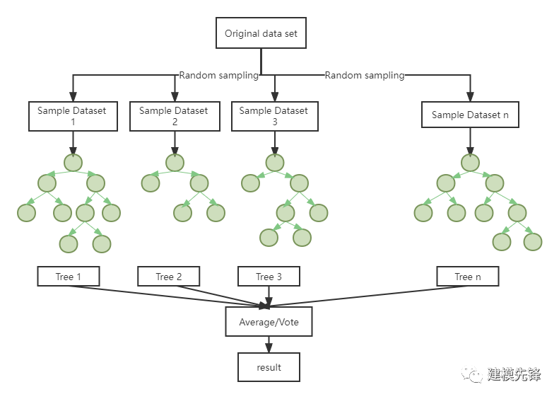
import pandas as pdimport numpy as npfrom sklearn.ensemble import RandomForestClassifier # 随机森林分类from sklearn.model_selection import train_test_split,GridSearchCV,cross_val_scorefrom sklearn.metrics import accuracy_score # 引入准确度评分函数from sklearn.metrics import mean_squared_errorfrom sklearn.metrics import confusion_matrix, accuracy_score,classification_reportfrom sklearn import preprocessingimport warningswarnings.filterwarnings('ignore')import matplotlib.pyplot as pltimport matplotlibmatplotlib.rc("font", family='Microsoft YaHei')
price_classify_data = pd.read_csv('yichang_deal.csv')X = price_classify_data[['zone_label','street_label','type_label','toward_label','area','floor_label','decorate_label','structure_label','follow']]Y = price_classify_data['price_label']# 标准化X = preprocessing.scale(X)X_train, X_test, Y_train, Y_test = train_test_split(X, Y, test_size=0.3, random_state=200) # 随机数种子
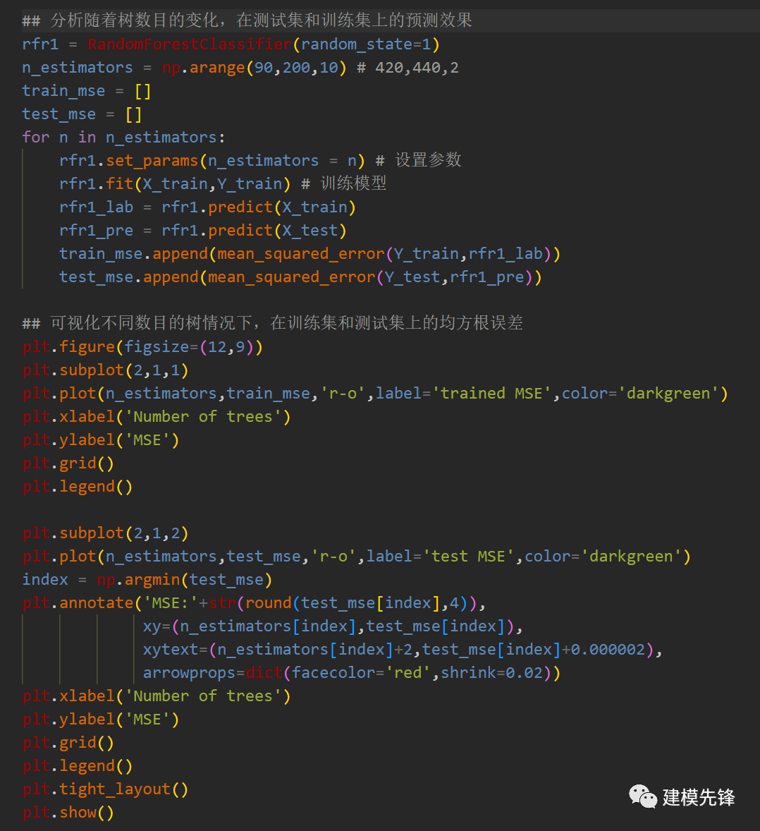
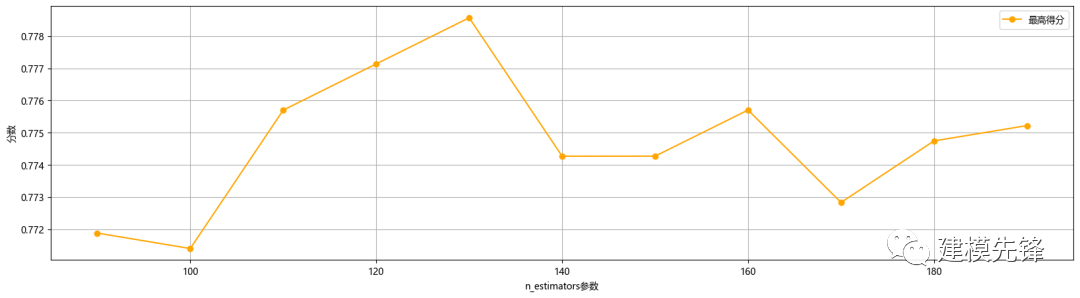
###调n_estimators参数ScoreAll = []for i in range(90,200,10):DT = RandomForestClassifier(n_estimators = i,random_state = 1) #,criterion = 'entropy'score = cross_val_score(DT,X_train,Y_train,cv=6).mean()ScoreAll.append([i,score])ScoreAll = np.array(ScoreAll)max_score = np.where(ScoreAll==np.max(ScoreAll[:,1]))[0][0] ##这句话看似很长的,其实就是找出最高得分对应的索引print("最优参数以及最高得分:",ScoreAll[max_score])plt.figure(figsize=[20,5])plt.plot(ScoreAll[:,0],ScoreAll[:,1],'r-o',label='最高得分',color='orange')plt.xlabel('n_estimators参数')plt.ylabel('分数')plt.grid()plt.legend()plt.show()# [130. 0.77857096]
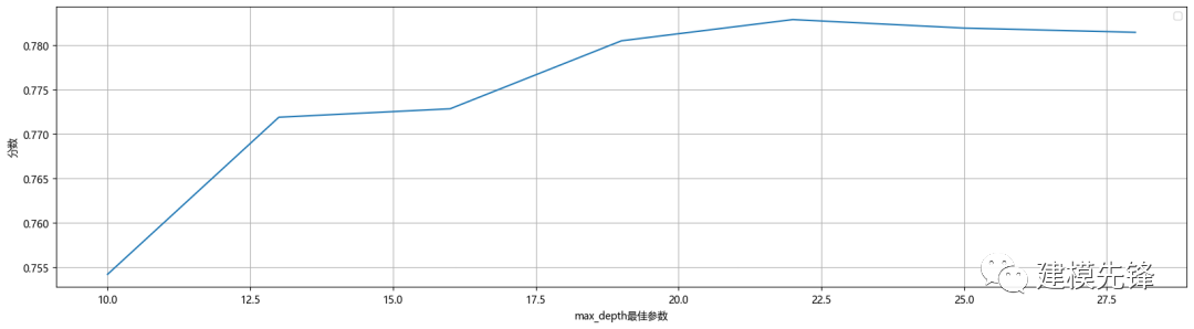
# 探索max_depth的最佳参数ScoreAll = []for i in range(10,30,3):DT = RandomForestClassifier(n_estimators = 130,random_state = 1,max_depth =i ) #,criterion = 'entropy'score = cross_val_score(DT,X_train,Y_train,cv=10).mean()ScoreAll.append([i,score])ScoreAll = np.array(ScoreAll)max_score = np.where(ScoreAll==np.max(ScoreAll[:,1]))[0][0]print("最优参数以及最高得分:",ScoreAll[max_score])plt.figure(figsize=[20,5])plt.plot(ScoreAll[:,0],ScoreAll[:,1])plt.xlabel('max_depth最佳参数')plt.ylabel('分数')plt.grid()plt.legend()plt.show()
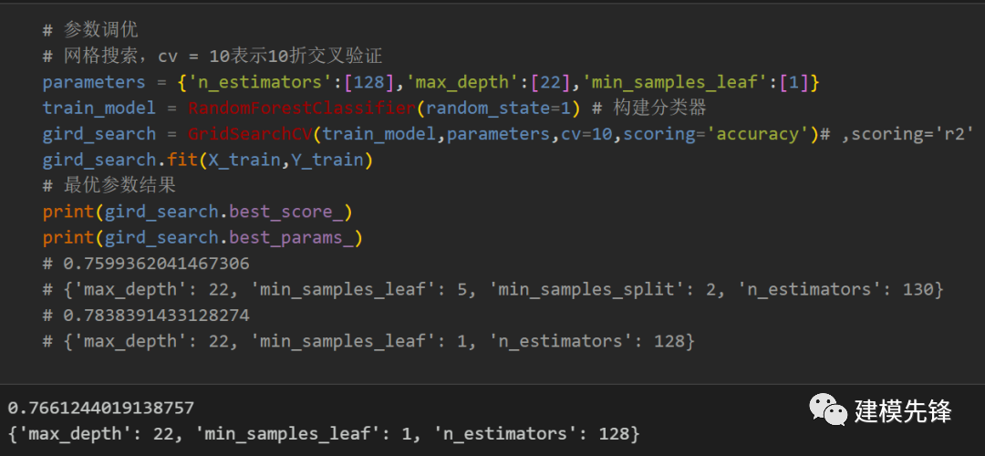
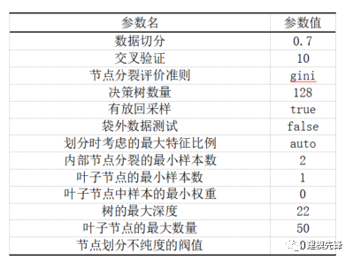
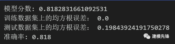
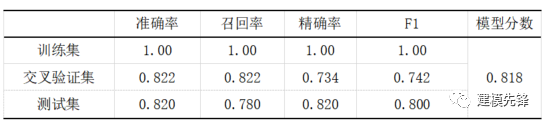
model = RandomForestClassifier(n_estimators=128,max_depth=22,random_state=1) # min_samples_leaf=11model.fit(X_train,Y_train)score = model.score(X_test,Y_test)print('模型分数:',score)# 计算在训练集和测试集上的预测均方根误差model_lab = model.predict(X_train)model_pre = model.predict(X_test)train_mse = mean_squared_error(Y_train,model_lab)test_mse = mean_squared_error(Y_test,model_pre)print('训练数据集上的均方根误差:',train_mse)print('测试数据集上的均方根误差:',test_mse)# 模型使用与评估y_pred = model.predict(X_test)print("准确率: %.3f" % accuracy_score(Y_test, y_pred))
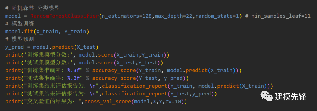
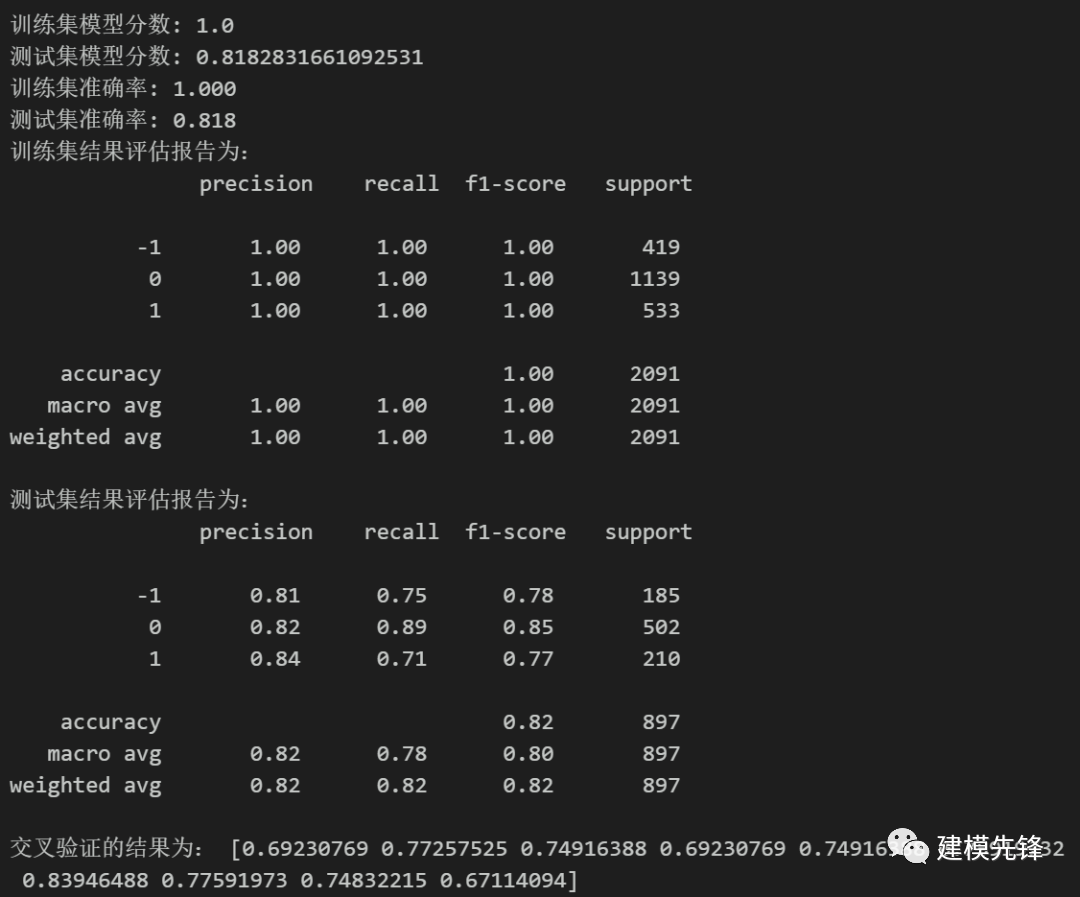
3模型评估
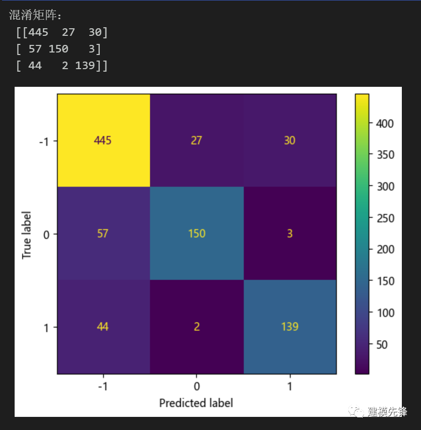
from sklearn.metrics import confusion_matriximport matplotlib.ticker as tickercm = confusion_matrix(Y_test, y_pred,labels=[0,1,-1])print('混淆矩阵:\n', cm)labels=['-1','0','1']from sklearn.metrics import ConfusionMatrixDisplaycm_display = ConfusionMatrixDisplay(cm,display_labels=labels).plot()# 混淆矩阵热力图def cm_plot(cm,labels):# 设置字体、字号plt.rc('font',family='Times New Roman',size='14')ind_array = np.arange(len(labels))x, y = np.meshgrid(ind_array, ind_array)for x_val, y_val in zip(x.flatten(), y.flatten()):# 转换为百分数,需同时更改colorbar标签(当然也可以直接以样本数表示,后续colorbar无需变动)c = round(cm[y_val][x_val]/sum(cm[y_val])*100,1)plt.text(x_val, y_val, c, color='b', va='center', ha='center')plt.imshow(cm, interpolation='nearest', cmap=plt.cm.binary)# colorbar设置cb = plt.colorbar()tick_locator = ticker.MaxNLocator(nbins=5)cb.locator = tick_locatorx_label = np.array(range(len(labels)))plt.xticks(x_label, labels)plt.yticks(x_label, labels, rotation=90)plt.ylabel('Actual label')plt.xlabel('Predict label')ax = plt.gca()tick_marks = np.array(range(len(labels))) + 0.5ax.set_xticks(tick_marks, minor=True)ax.set_yticks(tick_marks, minor=True)ax.xaxis.set_ticks_position('none')ax.yaxis.set_ticks_position('none')ax.grid(True, which='minor', linestyle='-')plt.tight_layout()plt.show()cm_plot(cm,labels)
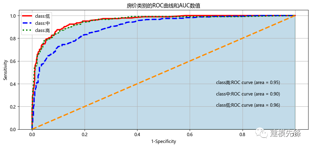
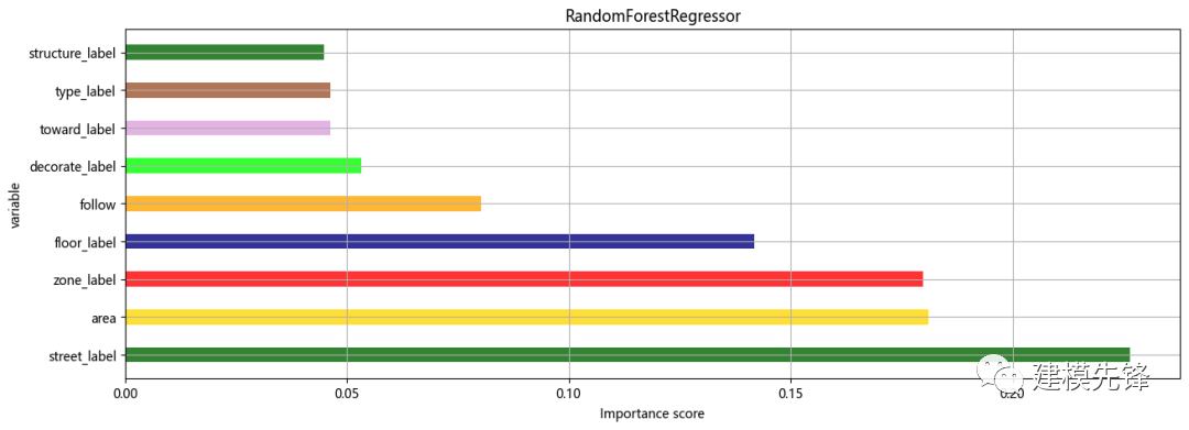
features = X.columnsimportances = model.feature_importances_df = pd.DataFrame()df['特征'] = featuresdf['重要性'] = importancesdf = df.sort_values('重要性',ascending=False)# df.iloc[2,1] = df.iloc[2,1]+0.2xx = df['特征']yy = df['重要性']colors = ['darkgreen','gold','red','navy','orange','lime','plum','sienna']plt.figure(figsize=(15,5))plt.barh(xx,yy,0.4,color=colors,alpha=0.8)#color参数传入颜色列表,可以在一幅图中显示不同颜色plt.xlabel('Importance score')plt.ylabel('variable')plt.title('RandomForestRegressor')plt.grid()plt.show()
点击下载:完整爬虫代码、房价数据、分类模型分析、回归预测模型分析代码

The End
发布于:2023-11-28,除非注明,否则均为原创文章,转载请注明出处。
还没有评论,来说两句吧...